![[*]](http://vismod.www.media.mit.edu/vismod/support/latex2html-98//cross_ref_motif.gif) is a typical human face, we
choose to use an average 3D face from a database of previously sampled faces
to obtain a smooth, mean 3D face. Figure shows a few of the
3D range data models we used to obtain the average 3D face.
is a typical human face, we
choose to use an average 3D face from a database of previously sampled faces
to obtain a smooth, mean 3D face. Figure shows a few of the
3D range data models we used to obtain the average 3D face.
In averaging the 3D faces in a database, we wish to see the mean 3D face converge to a stable structure as we introduce more sample 3D faces. We also expect the mean 3D face to be ``face-like'' in the sense that the averaging process will not smooth out its features to the point where they are no longer distinguishable. In other words, the mean 3D face should still have a nose, a mouth, eyes and so on. If we do not see this convergence and the mean face is a mere blob or ellipsoid, then our hypothesis is incorrect: the 3D structure of a human face is not regular enough to approximate multiple individuals. Another possible source of divergence is inadequate normalization before the averaging process. If the 3D faces in our database are not fully normalized before being averaged, then the mean face will not be face-like.
For each face in our 3D range data database, we manually select 4 points: the
left eye, the right eye, the nose and the mouth and note their 3D coordinates.
Each model in the database undergoes a 3D transformation with a vertical
stretch to map its 4 anchor points to the same destination set of anchor
points. Mathematically, the four 3D anchor points:
![]() for each model, are mapped to a
destination set of 3D anchor points:
for each model, are mapped to a
destination set of 3D anchor points:
![]() .
This mapping is given in
Equation where matrix T is defined as follows:
.
This mapping is given in
Equation where matrix T is defined as follows:
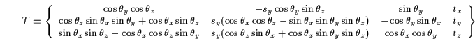 |
Using ten 3D models, the best transformation matrix was found by optimizing the
7 parameters
![]() to
minimize the fitting error, Efit as defined in Equation
below. There are 3 translation parameters
(tx,ty,tz), 3 rotation
parameters
to
minimize the fitting error, Efit as defined in Equation
below. There are 3 translation parameters
(tx,ty,tz), 3 rotation
parameters
![]() and one vertical stretch
parameter (sy):
and one vertical stretch
parameter (sy):
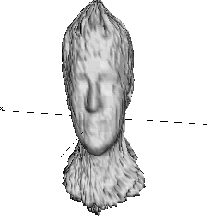
The final average 3D face range model is shown in Figure .
This is the only model that will be rotated, translated and deformed to
approximate the structure of new faces and the other 10 database models are
now discarded. As can be seen, the 3D mean face is a smooth, face-like
structure with distinct features. The coordinates of the features (eyes, nose
and mouth) are stored with the 3D model as
![]() for later use.
for later use.
![\begin{figure}\center
\begin{tabular}[b]{ccc}
\epsfig{file=norm/figs/alba.ps,...
...,height=4cm}\\
(a) & (b) & (c)
\end{tabular} \\ \vspace*{0.5cm}
\end{figure}](img136.gif)