


Next: Limb Length and Intensity
Up: Mouth Localization
Previous: Horizontal Symmetry Projection
Kelly proposes the linking of adjacent points in the axial symmetry maps as a
means of recovering complete limb structures from symmetry data
[20]. This process is simplified when only horizontally aligned
symmetry lines are to be considered since limb extraction is reduced to a 3
dimensional linking process. Limb extraction involves grouping points that are
adjacent in the
 space into continuous lines. However, since we
are only considering the horizontally projected symmetry lines, we only need
to connect points in a (x,y,r) space. Adjacent points in the axial symmetry
maps are linked using connected components analysis. Note that adjacent not
only refers to spatial adjacency but also adjacency in scale-space (i.e,
neighbouring values of r).
Since we are searching specifically for mouths, the connected component
analysis can be further constrained. Not only is the symmetry data projected
onto the horizontal, it is to be linked horizontally as well. We are searching
specifically for connected horizontal limbs and not an arbitrary cloud of
adjacent points from the images in Figure ![[*]](http://vismod.www.media.mit.edu/vismod/support/latex2html-98//cross_ref_motif.gif) . The extraction will
produce a set of 3D curves that flow through the symmetry data in
Figure
. The extraction will
produce a set of 3D curves that flow through the symmetry data in
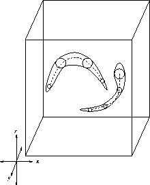
Figure ![[*]](http://vismod.www.media.mit.edu/vismod/support/latex2html-98//cross_ref_motif.gif) . Figure
. Figure ![[*]](http://vismod.www.media.mit.edu/vismod/support/latex2html-98//cross_ref_motif.gif) displays the limb axes
(shown with dashed lines) that should approximate the clouds (or manifolds) of
symmetry points (enclosed with continuous lines) in the search space.
displays the limb axes
(shown with dashed lines) that should approximate the clouds (or manifolds) of
symmetry points (enclosed with continuous lines) in the search space.
Figure 3.18:
Limb extraction
 |
Furthermore, these 3D curves are to be as horizontal as possible and should
not meander excessively. The mouth is a smooth limb so its axis should be
a simple straight line or a slight curve. Furthermore, axial symmetry curves
should not undulate excessively in scale-space, r (the third dimension).
This prevents the vertical thickness of the mouth limb from varying wildly. Thus,
mouth limbs which are maximally straight will be favored.
Figure ![[*]](http://vismod.www.media.mit.edu/vismod/support/latex2html-98//cross_ref_motif.gif) displays limb extractions which do not satisfy
these criteria and hence are probably not mouths. Such limbs should be
attenuated during extraction so that they will not interfere with mouth
detection. This attenuation agrees with the Gestalt psychology notion of
``Pragnanz'' which identifies a correspondence between simplicity in image
structures and their perceptual significance [3].
displays limb extractions which do not satisfy
these criteria and hence are probably not mouths. Such limbs should be
attenuated during extraction so that they will not interfere with mouth
detection. This attenuation agrees with the Gestalt psychology notion of
``Pragnanz'' which identifies a correspondence between simplicity in image
structures and their perceptual significance [3].
Figure 3.19:
Excessive limb undulation.
(a) Excessive spatial meandering. (b) Excessive meandering in scale
space.
![\begin{figure}\center
\begin{tabular}[b]{cc}
\epsfig{file=locs/figs/spatialMea...
...eight=2cm, angle=-90}\\
(a) & (b)
\end{tabular}\\ \vspace*{0.5cm}
\end{figure}](img103.gif) |
Connected component analysis begins at a given point (p,r) in the 3D search
space. This 3D search space covers values r=1 to r=6 and the (x,y)region depicted in Figure ![[*]](http://vismod.www.media.mit.edu/vismod/support/latex2html-98//cross_ref_motif.gif) . This starting point ((p,r) or
(x,y,r)) will be called the ``seed''. One of the requirements we impose is
that the seed has a significant horizontal symmetry magnitude (25% of the
maximum possible magnitude). From this starting point, we form a limb or 3D
curve by propagating along two trajectories: to the left and to the right.
. This starting point ((p,r) or
(x,y,r)) will be called the ``seed''. One of the requirements we impose is
that the seed has a significant horizontal symmetry magnitude (25% of the
maximum possible magnitude). From this starting point, we form a limb or 3D
curve by propagating along two trajectories: to the left and to the right.
By left propagation, we seek a path towards the left of the current pixel
(p,r) which flows through the strongest horizontal symmetry points in our 3D
search space. Along the left propagation, we utilize a kernel that covers all
the adjacent neighbours of the current point
(p,r)=(x,y,r) to the left of
the current pixel. This kernel is depicted in Figure ![[*]](http://vismod.www.media.mit.edu/vismod/support/latex2html-98//cross_ref_motif.gif) . This
kernel contains 9 cells of which we must pick one. This new cell becomes the
new ``current cell'' and we repeat the process, tracing out the next step in
the path from the 9 possible choices in the kernel. This propagation is
continued and the trajectory flows through the 3D space as it repeatedly
selects from the 9 possible cells in the kernel.
. This
kernel contains 9 cells of which we must pick one. This new cell becomes the
new ``current cell'' and we repeat the process, tracing out the next step in
the path from the 9 possible choices in the kernel. This propagation is
continued and the trajectory flows through the 3D space as it repeatedly
selects from the 9 possible cells in the kernel.
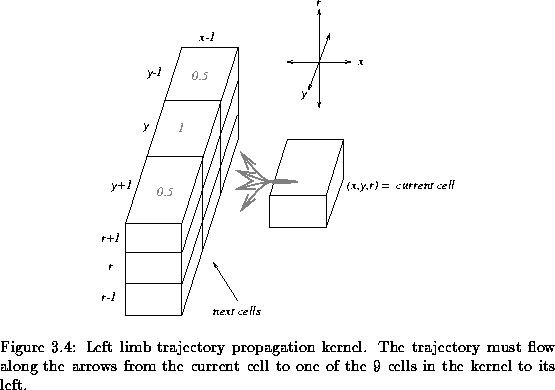
The symmetry magnitudes are scaled by the weights depicted in the kernel in
Figure ![[*]](http://vismod.www.media.mit.edu/vismod/support/latex2html-98//cross_ref_motif.gif) . We thus measure a weighted symmetry value from the
horizontal projection data for each cell in the kernel. The pixel location to
the immediate left is favored most and its symmetry magnitude is consequently
scaled by
. We thus measure a weighted symmetry value from the
horizontal projection data for each cell in the kernel. The pixel location to
the immediate left is favored most and its symmetry magnitude is consequently
scaled by  .
We simultaneously disfavor diagonally positioned pixels
by scaling their magnitude by
  .
We begin by only considering the
spatial neighbourhood at scale r. The peak weighted response from the three
cells at r is determined. If it is greater than the threshold (25%) then we
move (propagate) to the strongest cell's position and re-compute the kernel
from there. If on the other hand, the scale at r has only weak symmetry, we
repeat the analysis at r+1 and r-1 and propagate to the strongest of those
6 cells. Thus, we seek a path towards the left of the current pixel which
flows through the strongest horizontal symmetry. However, we favor paths that
are horizontal (limiting spatial meandering) and paths that are at the same
scale (limiting meandering in scale). Equation
 ![[*]](http://vismod.www.media.mit.edu/vismod/support/latex2html-98//cross_ref_motif.gif) illustrates the
weighted computation of the peak-response of the strongest cell in the kernel.
The cell generating the peak-response, peak is the one we move to next. It
becomes the ``current cell'' and we repeat the kernel computation from there.
The process stops when a dead end is reached and none of the 9 possible cells
contain an output greater than the threshold (25%). In
Equation
illustrates the
weighted computation of the peak-response of the strongest cell in the kernel.
The cell generating the peak-response, peak is the one we move to next. It
becomes the ``current cell'' and we repeat the kernel computation from there.
The process stops when a dead end is reached and none of the 9 possible cells
contain an output greater than the threshold (25%). In
Equation ![[*]](http://vismod.www.media.mit.edu/vismod/support/latex2html-98//cross_ref_motif.gif) , the horizontal symmetry values are labelled S where
S(x,y,r)=Srhorizontal(x,y).
, the horizontal symmetry values are labelled S where
S(x,y,r)=Srhorizontal(x,y).
 |
|
|
(3.3) |
A similar propagation is performed to the right of the seed (or starting cell)
and the two trajectories are merged into one. This single trajectory in the
spatial and scale domain represents the extracted limb as a whole.
Figure 3.21:
Search space for seeding mouth limb extraction
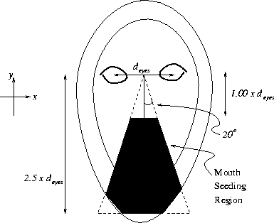 |
Figure ![[*]](http://vismod.www.media.mit.edu/vismod/support/latex2html-98//cross_ref_motif.gif) shows (in black) the (x,y) region in the image
where the mouth limb starting points will be selected. The dimensions of this
triangular search region are defined in the figure. Note that the triangle
does not extend beyond the face mask so that the mouth search is performed
exclusively within the face contour. Any part of the mouth that intersects
this triangular search space will trigger limb extraction. Thus, the mouth
does not have to be perfectly centered upon the face's mid-line. This can
happen if the face has an unusual pose or the eye detection is slightly
inaccurate. The triangular search space is superimposed upon the rotated
intensity image in Figure
shows (in black) the (x,y) region in the image
where the mouth limb starting points will be selected. The dimensions of this
triangular search region are defined in the figure. Note that the triangle
does not extend beyond the face mask so that the mouth search is performed
exclusively within the face contour. Any part of the mouth that intersects
this triangular search space will trigger limb extraction. Thus, the mouth
does not have to be perfectly centered upon the face's mid-line. This can
happen if the face has an unusual pose or the eye detection is slightly
inaccurate. The triangular search space is superimposed upon the rotated
intensity image in Figure ![[*]](http://vismod.www.media.mit.edu/vismod/support/latex2html-98//cross_ref_motif.gif) . Observe how the mouth is
not perfectly aligned with the face's mid-line in
Figure
. Observe how the mouth is
not perfectly aligned with the face's mid-line in
Figure ![[*]](http://vismod.www.media.mit.edu/vismod/support/latex2html-98//cross_ref_motif.gif) . However, it still falls within the generous
triangular search region and is thus detectable.
. However, it still falls within the generous
triangular search region and is thus detectable.
Figure 3.22:
Search space for mouth superimposed on face
 |
Note that this triangular search space is rather redundant. Say a horizontal
limb is detected at a seed position (x,y,r) on the image. A very similar
limb will probably be detected when we start the limb extraction at
(x+1,y,r). Thus, we do not need to start the limb extraction process at
every point in the triangle. We merely start the limb extraction once for
every value of y in the triangle. For each value of y we select the seeding point
(x,y,r) by varying x and r to maximize
Srhorizontal(x,y). Then,
we begin the limb extraction and extract via propagation the trajectory of the
limb towards the left and the right. This is repeated for each value of y in
the triangle resulting in a collection of limb axes.
Figure 3.23:
Limb axes extracted as 3D trajectories
![\begin{figure}\center
\begin{tabular}[b]{cc}
\epsfig{file=locs/figs/limb.ps,he...
...limbs2.ps,height=2cm, angle=-90}\\
\end{tabular}\\ \vspace*{0.5cm}
\end{figure}](img109.gif) |
The resulting horizontal limb axes are stored as 3D curves (or trajectories)
in the spatial-scale domain as shown in Figure ![[*]](http://vismod.www.media.mit.edu/vismod/support/latex2html-98//cross_ref_motif.gif) . The height in
this graph represents the scale or the dimension r of the trajectory. This
value of r corresponds directly to the thickness of the limb being
extracted. Now, we must test these limbs to determine which of them is the
mouth. Some particularly short limbs are present in Figure
. The height in
this graph represents the scale or the dimension r of the trajectory. This
value of r corresponds directly to the thickness of the limb being
extracted. Now, we must test these limbs to determine which of them is the
mouth. Some particularly short limbs are present in Figure ![[*]](http://vismod.www.media.mit.edu/vismod/support/latex2html-98//cross_ref_motif.gif) despite the Gaussian filtering. These limbs will be discarded later since they
are too short.
despite the Gaussian filtering. These limbs will be discarded later since they
are too short.


Next: Limb Length and Intensity
Up: Mouth Localization
Previous: Horizontal Symmetry Projection
Tony Jebara
2000-06-23
![[*]](http://vismod.www.media.mit.edu/vismod/support/latex2html-98//cross_ref_motif.gif) . The extraction will
produce a set of 3D curves that flow through the symmetry data in
Figure
. The extraction will
produce a set of 3D curves that flow through the symmetry data in
Figure ![[*]](http://vismod.www.media.mit.edu/vismod/support/latex2html-98//cross_ref_motif.gif) . Figure
. Figure ![[*]](http://vismod.www.media.mit.edu/vismod/support/latex2html-98//cross_ref_motif.gif) displays the limb axes
(shown with dashed lines) that should approximate the clouds (or manifolds) of
symmetry points (enclosed with continuous lines) in the search space.
displays the limb axes
(shown with dashed lines) that should approximate the clouds (or manifolds) of
symmetry points (enclosed with continuous lines) in the search space.

![\begin{figure}\center
\begin{tabular}[b]{cc}
\epsfig{file=locs/figs/spatialMea...
...eight=2cm, angle=-90}\\
(a) & (b)
\end{tabular}\\ \vspace*{0.5cm}
\end{figure}](img103.gif)


![\begin{figure}\center
\begin{tabular}[b]{cc}
\epsfig{file=locs/figs/limb.ps,he...
...limbs2.ps,height=2cm, angle=-90}\\
\end{tabular}\\ \vspace*{0.5cm}
\end{figure}](img109.gif)