Understanding and predicting the appearance of outdoor scenes under arbitrary lighting and weather conditions is a fundamental problem in computer vision and computer graphics. Solutions to this problem have implications for several application domains including image-based rendering, remote sensing, and visual surveillance. The appearance of an outdoor scene is highly complex and depends on factors such as viewing direction, scene structure and material properties (sand, brick, grass), illumination (sun, moon, stars, street lamps), atmospheric condition (clear air, haze, mist, fog, rain) and aging (patina, corrosion, rust) of materials. Over time, these factors change, altering the way a scene appears. A large set of images is required to study the entire variability in scene appearance. The Columbia Weather and Illumination Database (WILD) is being collected for this purpose.
The WILD database consists of high quality (1520 x 1008 pixels, 12 bits per pixel) calibrated color (RGB) images of an outdoor scene captured every hour for over 6 months. The data collection is ongoing and we plan to acquire images for one year. The dataset covers a wide range of daylight and night illumination conditions, weather conditions and all 4 seasons. This webpage describes in detail the image acquisition and sensor calibration procedures. The images are tagged with a variety of ground truth data such as atmospheric conditions (weather, visibility, sky condition, humidity, temperature) and approximate scene depths. |
The Scene
The scene we image is an urban scene in uptown Manhattan with buildings, trees and sky. The distances of these buildings range from about 20 meters to about 5 kilometers. The large distance range facilitates the observation of weather effects on scene appearance. See Figure for the entire field of view.
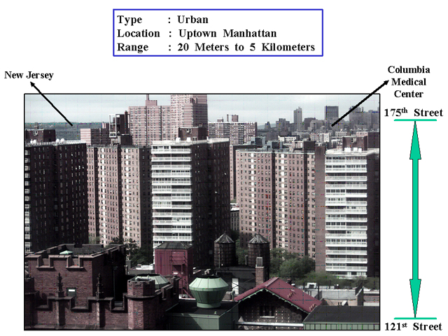 |
Image Quality, Quantity and Format
Images are captured automatically every hour for 20 hours each day (on an average). The spatial resolution of each image is 1520 x 1008 pixels and the intensity resolution is 10 bits per pixel per color channel. Currently, we have acquired images for over 150 days. In total, the database has around 3000 images.
To capture both subtle and large changes in illumination and weather, high dynamic range images are required. So, the images are acquired with multiple exposures (by changing the camera shutter speed while keeping the aperture constant) and apply existing techniques to compute a high dynamic range image (approx. 12 bits per pixel per color channel) of the scene. See the section on calibration for more details.
The images are stored in uncompressed 48-bit RGB tif format which can be read using software such as Photoshop, xv, or matlab.
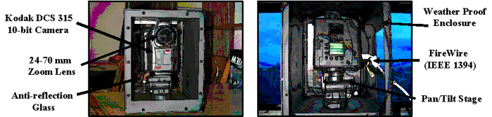
Acquisition Hardware
The digital camera used for image capture is a single CCD KODAK Professional DCS 315 (see Figure). As usual, irradiance is measured using 3 wideband R, G, and B color filters. An AF Nikkor 24 mm - 70 mm zoom lens is attached to the camera. The setup for acquiring images is shown in Figure. The camera is rigidly mounted over a pan-tilt head which is fixed rigidly to a weather-proof box. The weather-proof box is coated on the inside with two coats of black paint to prevent inter-reflections within the box. An anti-reflection glass plate is attached to the front of this box through which the camera views the scene. Between the camera and the anti-reflection plate, is a filter holder (for, say, narrow band spectral filters). The entire box with the camera and the anti-reflection glass plate is mounted on a panel rigidly attached to a window.
Calibration
The various calibration and preprocessing steps performed on the image set are as follows:
| |
Geometric Calibration
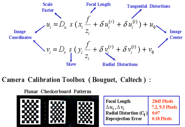
Geometric calibration constitutes the estimation of the geometric mapping between 3D scene points and their image projections. Since the calibration was done in a location different from that used for image acquisition, only the intrinsic parameters of the camera are estimated. Intrinsic parameters include the effective focal length, f, skew, s, center of projection (u0, v0) and distortion parameters, C1 ... Cn (radial) and P1, P2 (tangential).
The images of a planar checkerboard pattern were captured under various orientations (see figure). The corresponding corners of the checkerboard patterns in these images were marked. These corresponding corner points were input to a calibration routine [1] to obtain the intrinsic parameters. The table shows the estimated intrinsic parameters. The CCD pixels are square and hence skew is assumed to be 1. The deviation of the principal point from the image center is given by u0, v0. Only the first radial distortion parameter, C1, is shown. The remaining distortion parameters are set to zero.
 |
Radiometric Response Function
Analysis of image irradiance using measured pixel brightness requires the radiometric response of the sensor. The radiometric response of a sensor is the mapping, g, from image irradiance, I, to measured pixel brightness, M : M = g(I) Then, the process of obtaining I from M: I = g^(-1)(M) upto a global scale factor, is termed as radiometric calibration.
Radiometric Calibration
The response functions of CCD cameras (without considering the gamma or color corrections applied to the CCD readouts) are close to linear. The response functions were computed for the 3 RGB channels separately using Mitsunaga and Nayar's [2] radiometric self-calibration method. In this method, images captured with multiple exposures and the their relative exposure values are used to estimate the inverse response function in polynomial form. The results of the calibration are shown in the plots of the figure. Notice that the response functions of R, G, and B are linear and they have different slopes - 1.5923, 1.005 and 0.982 respectively. To balance the colors, we normalize the response functions by the respective slopes.
| | |