HW4 - 3101 Matlab -- (INSERT NAME and UNI HERE)

Due 11:59pm on Tuesday, April 8th, 2008

Goals
Directions
Problem 1 - Conway's Game of Life
1.1
1.1.2
1.1.3
1.1.4
1.2
1.3
1.4
1.4.1
1.4.2
Problem 2 -- Image Filters
2.1
2.1.1
2.1.2
2.2
2.2.1
2.2.2
2.2.3
2.2.4
2.3
2.3.1
2.3.2
2.3.3
Problem 3 - Where's Waldo with Template Matching
3.1
3.2
3.3
3.4
3.5
3.6

Goals

Working with graphics, simple animation, and images

Directions

Please fill in your name at the top of this page and write your answers under their corresponding question. When you are done, publish this file to html using File > Publish To HTML (or the command publish('hw1.m', 'html') and create a new zip file that is labeled with your UNI and homework number, in this format: bs2018_hw1.zip, that contains this original m file, and the html directory created from publishing the file. Make sure the html file adequately shows your work, (has images, etc.), and then email this file to cs3101@gmail.com, making sure to include your name, and uni in the subject.

Problem 1 - Conway's Game of Life

Conway's Game of Life is a cellular automation that operates on a 2D grid. Life is a wonderful example of how complex patterns can arise from very simple rules and initial conditions.

N = 20;

1.1

Using only one command. Make a grid of size NxN where 80% of the entries are randomly set to 1 and the rest are zero. Store the grid in the variable X. Do not display X.

X = rand(N, N) > 0.8;

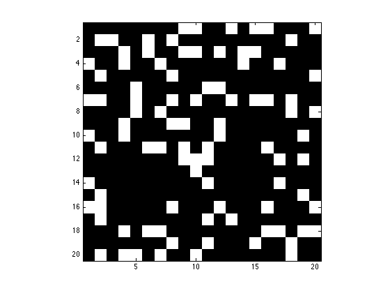
1.1.2

Change the colormap to black and white and display X in figure 1, make sure to change the axis so that X is displayed as square.

figure(1); imagesc(X); axis image; drawnow;
colormap('gray');

1.1.3

For each cell of the grid, count how many of its 8 neighbors are equal to 1. Store the number of neighbors for each cell in a new variable called neighbors. The grid should be connected left to right and top to bottom, so that it's continuous. Cells on the boundary on the right for example may have neighbors on the left boundary. Hint: it's much simpler to do this with one big command, and it involves circularly shifting around and adding the original matrix X.

neighbors = circshift(X, [1, 0]) + circshift(X, [-1, 0]) +  circshift(X, [0, 1]) +  circshift(X, [0, -1]) + ...
circshift(X, [1, 1]) + circshift(X, [-1, 1]) + circshift(X, [1, -1]) + circshift(X, [-1, -1]);

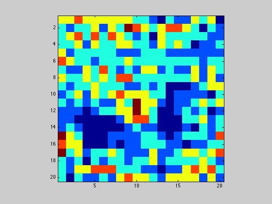
1.1.4

Display neighbors as a heatmap in figure 2 using the colormap jet

figure(2); imagesc(neighbors); axis image; drawnow;
colormap('jet');

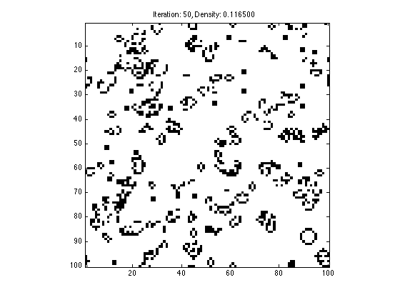
1.2

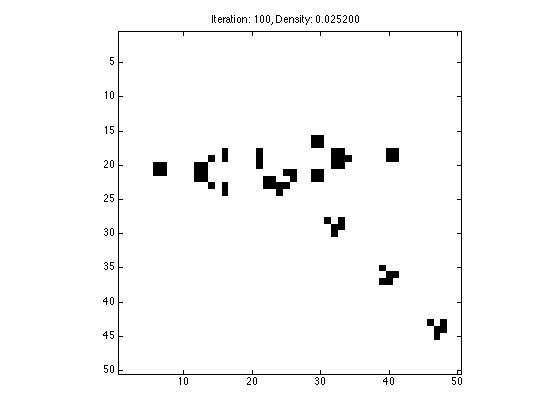
Implement and run conway's game of life on a 100x100 grid where initially 80% of the entries are randomly assigned to 1. Some notes:

Only run 50 iterations of conways game of life and then stop
Neighbors are computed as stated above (the grid wraps around itself like a torus)
At each iteration plot the grid in figure 1, so you can see it animate, but plot white for 0s and black for 1s
Make the title for figure 1 show which iteration the simulation is at, and the percentage of cells which are equal to 1

N = 100;
T = 50;


X = rand(N, N) > 0.5;

figure(1); imagesc(X); axis image; colormap gray; drawnow;
for t=1:T
    neighbors = circshift(X, [1, 0]) + circshift(X, [-1, 0]) +  circshift(X, [0, 1]) +  circshift(X, [0, -1]) + ...
    circshift(X, [1, 1]) + circshift(X, [-1, 1]) + circshift(X, [1, -1]) + circshift(X, [-1, -1]);

    X(find(((neighbors > 3) | (neighbors < 2))  & X)) = 0;
    X(find((neighbors == 3) & ~X)) = 1;

    figure(1); imagesc(1-X); axis image; colormap gray;
    title(sprintf('Iteration: %d, Density: %f', t, sum(sum(X))/(N*N)));
    drawnow;

end

1.3

Write a short piece of code that initializes an empty 50x50 grid, plots that grid in figure 1 and then prompts the user to click on the plot. The user is able to toggle the color of cells between black and white by clicking on them. Changing the color of the cell changes the underlying values in the grid from 1 to 0 and vice versa. The user should be able to terminate the loop by right-clicking anywhere without making a dot (the dots are made by left clicks).

NOTE: before you publish your HW, you must comment out this code because it is interactive, but to prove that it works you will use this bit of code in the next question.

% N = 50;
% X = zeros(N, N);
% colormap gray;
% figure(1); imagesc(1 - X); axis image; drawnow;
% but=1;
%
% while but==1
%     figure(1);
%     [a, b, but] = ginput(1);
%     yi = round(a);
%     xi = round(b);
%
%     if but==1
%         if X(xi, yi)
%             X(xi, yi) = 0;
%         else
%              X(xi, yi) = 1;
%         end
%     end
%
%     figure(1); imagesc(1 - X); axis image; colormap gray; drawnow;
% end

1.4

Use the piece of code you wrote above to draw Gosper's Glider Gun. When you have sucessfully done it once. Save X (your grid) to a file called Xgosperglider.mat (only save the one variable X to this file). Comment out the interactive code above, and simply load the .mat file below, and apply conways game of life to it. Only run Life for 100 iterations.

load Xglidergun.mat;
X = Xglidergun;
N = length(X);
T = 100;

figure(1); imagesc(X); axis image; colormap gray; drawnow;
for t=1:T
    neighbors = circshift(X, [1, 0]) + circshift(X, [-1, 0]) +  circshift(X, [0, 1]) +  circshift(X, [0, -1]) + ...
    circshift(X, [1, 1]) + circshift(X, [-1, 1]) + circshift(X, [1, -1]) + circshift(X, [-1, -1]);

    X(find(((neighbors > 3) | (neighbors < 2))  & X)) = 0;
    X(find((neighbors == 3) & ~X)) = 1;

    figure(1); imagesc(1-X); axis image; colormap gray;
    title(sprintf('Iteration: %d, Density: %f', t, sum(sum(X))/(N*N)));
    drawnow;

end

1.4.1

Figure 1 should currently contain your Gosper Glider Gun after it has been iterated with life 100 times. Write this entire figure window to an image file called 'gliderFigure.png'. Make sure you write the entire figure, with the title, etc.

saveas(gcf, 'myGosperGliderFigure.png');

1.4.2

Now simply write to an image file for the data which is contained inside the plot (the data in variable X). This image should be 50x50 pixels, and does not contain the axes or the title.

imwrite(1-X, 'myGosperGlider.png', 'png');

Problem 2 -- Image Filters

2.1

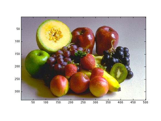
Download the image fruit.jpg from the class website, and load the image into a variable called X.

X = importdata('fruit.jpg');

2.1.1

Display X in figure 1, make sure sure the axes are set so that pixels are square

imagesc(X); axis image;

2.1.2

What are the dimensions of X?

size(X)

ans =

   333   500     3

2.2

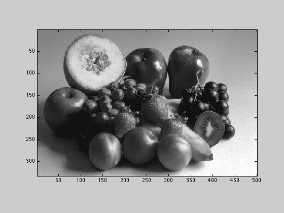
A grayscale image can be computed by averaging the red, green, and blue components for each pixel. Convert X to grayscale and store that result in variable called Xbw.

Xbw = mean(X, 3);

2.2.1

Display Xbw twice, once using the gray colormap,

figure(2); imagesc(Xbw); axis image; colormap('gray');

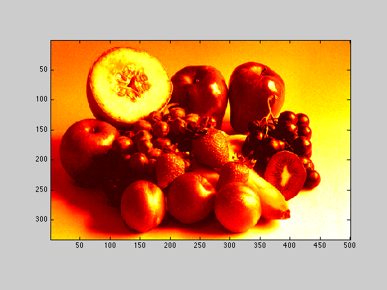
2.2.2

Display Xbw using the hot colormap

figure(2); imagesc(Xbw); axis image; colormap('hot');

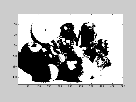
2.2.3

Compute and show a new image called Xthresh, which is white wherever the intesity of Xbw is greater then 85 and black everywhere the intensity is less then 85.

Xthresh = Xbw;
t = 85;
Xthresh(Xthresh < t) = 0;
Xthresh(Xthresh > t) = 255;

figure(2); imagesc(Xthresh); axis image; colormap('gray');

2.2.4

write the Xthresh image out as a png. do not write the whole figure window, just the image.

imwrite(Xthresh, 'fruitbw.png', 'png');

2.3

The Sobel Operator is a way to do edge detection and is used in many computer vison applications. Print out the help for conv2, and read through the wikipedia article on the Sobel Operator

help conv2

 CONV2 Two dimensional convolution.
    C = CONV2(A, B) performs the 2-D convolution of matrices
    A and B.   If [ma,na] = size(A) and [mb,nb] = size(B), then
    size(C) = [ma+mb-1,na+nb-1].
 
    C = CONV2(H1, H2, A) convolves A first with the vector H1 
    along the rows and then with the vector H2 along the columns.
 
    C = CONV2(..., SHAPE) returns a subsection of the 2-D
    convolution with size specified by SHAPE:
      'full'  - (default) returns the full 2-D convolution,
      'same'  - returns the central part of the convolution
                that is the same size as A.
      'valid' - returns only those parts of the convolution
                that are computed without the zero-padded
                edges. size(C) = [ma-mb+1,na-nb+1] when
                all(size(A) >= size(B)), otherwise C is 
                an empty matrix [].
 
    If any of A, B, H1, and H2 are empty, then C is 
    an empty matrix [].
 
    See also CONV, CONVN, FILTER2 and, in the Signal Processing
    Toolbox, XCORR2.

    Overloaded functions or methods (ones with the same name in other directories)
       help uint8/conv2.m
       help uint16/conv2.m

    Reference page in Help browser
       doc conv2

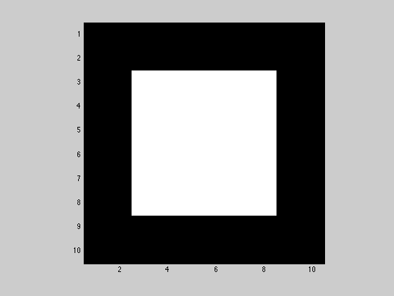
2.3.1

Create a new variable A that is 10x10 and contains all zeros except for the middle 6x6 elemnts which contain ones. Display A as a grayscale image.

figure(3);
A = zeros(10);
A(3:8,3:8) = ones(6);
imagesc(A); axis image; colormap('gray');

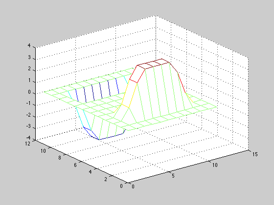
2.3.2

Compute Gx by convolving the sobel kernel with the A matrix. Display Gx as a mesh in figure 4 with the colormap jet.

sobel = [1, 2, 1; 0, 0, 0; -1, -2, -1];

Gx = conv2(A,sobel);

figure(5); mesh(Gx); colormap('jet');

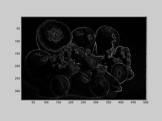
2.3.3

Compute Gx, Gy, and G for the fruit image by following how it is done in the wikipedia article. Display the result as an image. Save the result to a png file.

sobel = [1, 2, 1; 0, 0, 0; -1, -2, -1];

Gx = conv2(Xbw,sobel);
Gy = conv2(Xbw ,sobel');
G = sqrt(Gx.^2 + Gy.^2);

G = uint8(255 * G ./ max(max(G)));

imagesc(G); axis image; colormap('gray');

imwrite(G, 'fruitsobel.png', 'png');

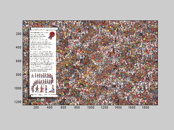
Problem 3 - Where's Waldo with Template Matching

3.1

load the two images waldo.png, and findwaldobig.jpg.

template = importdata('waldo.png');
im = importdata('findwaldobig.jpg');

3.2

Display findwaldobig

imagesc(im); axis image;

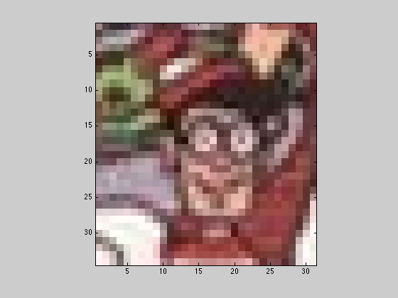
3.3

Display waldo

imagesc(template); axis image;

3.4

Print out the help pages for normxcorr2

help normxcorr2

 NORMXCORR2 Normalized two-dimensional cross-correlation.
    C = NORMXCORR2(TEMPLATE,A) computes the normalized cross-correlation of
    matrices TEMPLATE and A. The matrix A must be larger than the matrix
    TEMPLATE for the normalization to be meaningful. The values of TEMPLATE
    cannot all be the same. The resulting matrix C contains correlation
    coefficients and its values may range from -1.0 to 1.0.
 
    Class Support
    -------------
    The input matrices can be numeric. The output matrix C is double.
 
    Example
    -------
    template = .2*ones(11); % make light gray plus on dark gray background
    template(6,3:9) = .6;   
    template(3:9,6) = .6;
    BW = template > 0.5;      % make white plus on black background
    figure, imshow(BW), figure, imshow(template)
    % make new image that offsets the template
    offsetTemplate = .2*ones(21); 
    offset = [3 5];  % shift by 3 rows, 5 columns
    offsetTemplate( (1:size(template,1))+offset(1),...
                    (1:size(template,2))+offset(2) ) = template;
    figure, imshow(offsetTemplate)
    
    % cross-correlate BW and offsetTemplate to recover offset  
    cc = normxcorr2(BW,offsetTemplate); 
    [max_cc, imax] = max(abs(cc(:)));
    [ypeak, xpeak] = ind2sub(size(cc),imax(1));
    corr_offset = [ (ypeak-size(template,1)) (xpeak-size(template,2)) ];
    isequal(corr_offset,offset) % 1 means offset was recovered
 
   See also CORRCOEF.

    Reference page in Help browser
       doc normxcorr2

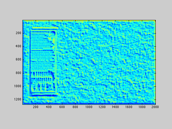
3.5

Convert the two images two grayscale, and run normxcorr2 on them to get a matrix of correlation values, the maximum of which, corresponds to the best place to put the smaller image so that it lines up with the big image. Call this matrix of correlations W, and display it using the jet heat map. Note: normxcorr2 could take a while to run.

template = mean(template, 3);
im = mean(im, 3);

W = normxcorr2(template, im);
imagesc(W); axis image; colormap('jet');

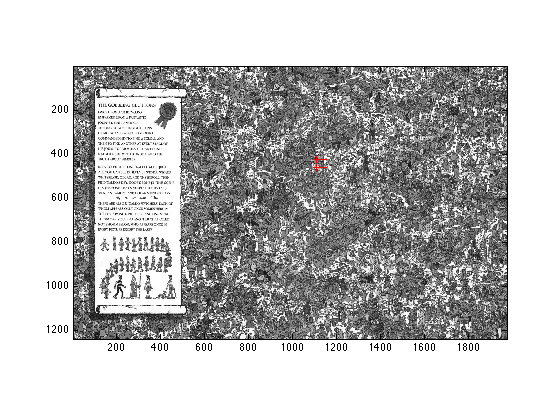
3.6

Find the coordinates for the maximum of W (display them), and use the hold, and scatter commands to plot the grayscale findwaldobig image, and plot 4 red dots around where you found waldo.

W1 = W(:);
size(W1);

[C, I] = max(W1);

figure(1); clf;
imagesc(im); axis image; colormap('gray');
hold on;

[y, x] = ind2sub(size(W), I)
scatter(x, y, 'r+');
scatter(x - size(template, 2), y, 'r+');
scatter(x, y - size(template, 1), 'r+');
scatter(x - size(template, 2), y - size(template, 1), 'r+');

hold off;