Programming Languages Matlab 3101 - Class 1
3/5/08, Instructor: Blake Shaw
Contents
- Overview
- How to get help
- Matlab as a calculator
- Mathematical functions
- Working with variables
- Using scripts -- running commands listed in a file
- Working with arrays
- Element wise operations with arrays
- Useful functions for working with arrays
- Indexing mutliple items in a arrays with the colon operator
- Different ways to index
- You can apply mathematical functions to arrays
- Other useful functions with arrays
- Numbers, Arrays, and Matrices... all the same
- Can do math with matrices
- Generating arrays and matrices
- Let's plot some stuff, it's easy!
- plotting sin
- histograms
- bar and pie plots
- More notes
Overview
Matlab as a calculator: mathematical functions, arrays, array operations, matrices, simple plotting tools, running script files
How to get help
help and doc
help sin
doc sin
 SIN    Sine of argument in radians.
    SIN(X) is the sine of the elements of X.

    See also ASIN, SIND.

    Overloaded functions or methods (ones with the same name in other directories)
       help darray/sin.m
       help sym/sin.m

    Reference page in Help browser
       doc sin
Matlab as a calculator
do some math!
a = 2 + 3 + 4
a = 3.156
a =

     9


a =

    3.1560
Mathematical functions
abs, factor, factorial,
abs(-10 * a)
ans =

   31.5600
Working with variables
declare variables, use them in equations, semi-colon suppresses output
a = 3;
b = 4;
c = sqrt(a^2 + b^2)
c =

     5
Using scripts -- running commands listed in a file
show how to make comments, use cell mode, cd into directory and run a file
Working with arrays
make an array from a list of numbers, and do some math on it
p = [1, 4, 5, 6, 8]

p * 2

factorial(p)
p =

     1     4     5     6     8


ans =

     2     8    10    12    16


ans =

           1          24         120         720       40320
Element wise operations with arrays
.* and * are different, this is tricky!
p .* p

p .^ 2
ans =

     1    16    25    36    64


ans =

     1    16    25    36    64
Useful functions for working with arrays
get the size of it, access elements of it, concatenate arrays remove elements
p

size(p)

p(3)


p2 = [p, 3]

p4 = [1, p, p, 5]

p(1) = [];
p =

     1     4     5     6     8


ans =

     1     5


ans =

     5


p2 =

     1     4     5     6     8     3


p4 =

     1     1     4     5     6     8     1     4     5     6     8     5
Indexing mutliple items in a arrays with the colon operator
the colon operator is great for indexing... really great...
1:5

10:20

100:105

p(2:4)
p([2, 3, 4])
ans =

     1     2     3     4     5


ans =

    10    11    12    13    14    15    16    17    18    19    20


ans =

   100   101   102   103   104   105


ans =

     5     6     8


ans =

     5     6     8
Different ways to index
binary vector, using end, different increments
10:-1:1
x = 2:7:20;

size(x)

i = logical([1, 0, 1]);

x(i)

isprime(x)
ans =

    10     9     8     7     6     5     4     3     2     1


ans =

     1     3


ans =

     2    16


ans =

     1     0     0
You can apply mathematical functions to arrays
more then just plus and minus
p + 3

p.^2 + 10
ans =

     7     8     9    11


ans =

    26    35    46    74
Other useful functions with arrays
sum, max, min, length, sort, mean, std, whos, clear, size
sum(p)
max(p)
min(p)

t = [-5, 6, 4, 2, 9, 1, 2, 4];

mean(t)
std(t)
sort(t)
ans =

    23


ans =

     8


ans =

     4


ans =

    2.8750


ans =

    4.0861


ans =

    -5     1     2     2     4     4     6     9
Numbers, Arrays, and Matrices... all the same
just different sizes...
A = [1, 2; 3, 4]
A =

     1     2
     3     4
Can do math with matrices
simple stuff like plus and minus, more complicated stuff like inverse, transpose, eig, diag,
A .^ 2

B = [A.^2, A.^3; A.^4, A.^5]

a =1:5

C = [a; a.^2; a.^3]
ans =

     1     4
     9    16


B =

           1           4           1           8
           9          16          27          64
           1          16           1          32
          81         256         243        1024


a =

     1     2     3     4     5


C =

     1     2     3     4     5
     1     4     9    16    25
     1     8    27    64   125
Generating arrays and matrices
colon is great, but also there is rand, ones, zeros, eye, etc...
D = rand(5, 5)

D = ones(5, 5)

D = zeros(5, 5)

D = eye(5, 5)
D =

    0.8147    0.0975    0.1576    0.1419    0.6557
    0.9058    0.2785    0.9706    0.4218    0.0357
    0.1270    0.5469    0.9572    0.9157    0.8491
    0.9134    0.9575    0.4854    0.7922    0.9340
    0.6324    0.9649    0.8003    0.9595    0.6787


D =

     1     1     1     1     1
     1     1     1     1     1
     1     1     1     1     1
     1     1     1     1     1
     1     1     1     1     1


D =

     0     0     0     0     0
     0     0     0     0     0
     0     0     0     0     0
     0     0     0     0     0
     0     0     0     0     0


D =

     1     0     0     0     0
     0     1     0     0     0
     0     0     1     0     0
     0     0     0     1     0
     0     0     0     0     1
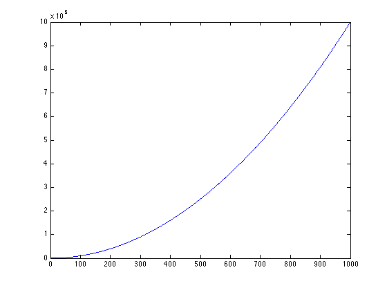
Let's plot some stuff, it's easy!
some basics of plotting, plot, hist, bar, pie
x = 1:1000;
y = x.^2;

x(1:5)
y(1:5)

plot(y)
ans =

     1     2     3     4     5


ans =

     1     4     9    16    25
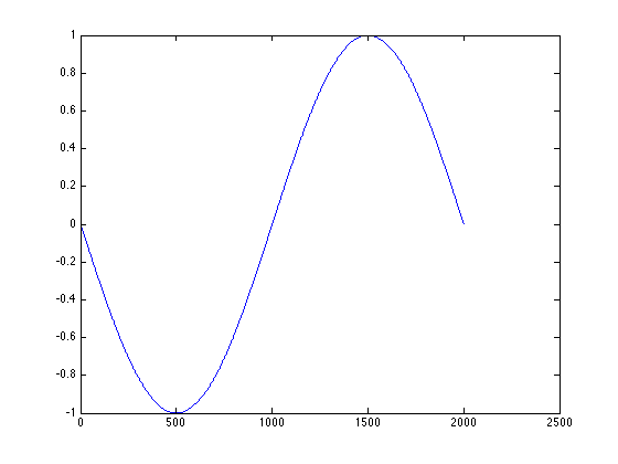
plotting sin
x = -pi:(pi/1000):pi;

y = sin(x);

size(x)

plot(y)
ans =

           1        2001
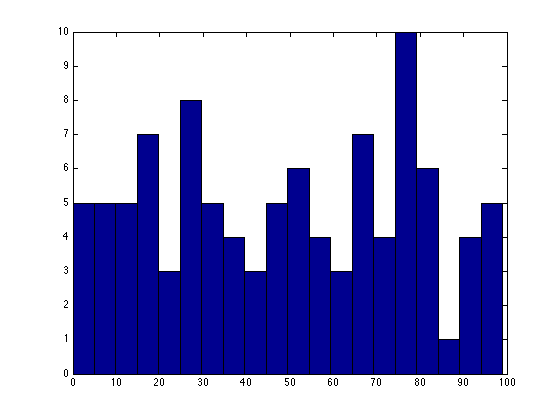
histograms
a = floor(100*rand(100, 1))

plot(a)
hist(a, 20)
a =

    75
    74
    39
    65
    17
    70
     3
    27
     4
     9
    82
    69
    31
    95
     3
    43
    38
    76
    79
    18
    48
    44
    64
    70
    75
    27
    67
    65
    16
    11
    49
    95
    34
    58
    22
    75
    25
    50
    69
    89
    95
    54
    13
    14
    25
    84
    25
    81
    24
    92
    34
    19
    25
    61
    47
    35
    83
    58
    54
    91
    28
    75
    75
    38
    56
     7
     5
    53
    77
    93
    12
    56
    46
     1
    33
    16
    79
    31
    52
    16
    60
    26
    65
    68
    74
    45
     8
    22
    91
    15
    82
    53
    99
     7
    44
    10
    96
     0
    77
    81
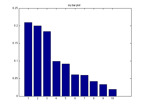
bar and pie plots
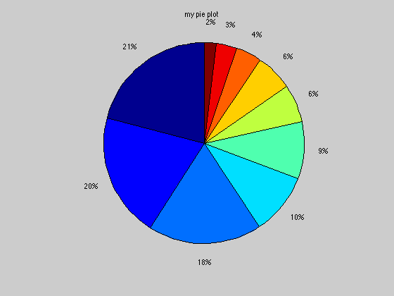
r = rand(10, 1)

sum(r)

r2 = r ./ sum(r)

sum(r2)

r3 = sort(r2, 'descend')

figure(1);
bar(r3)
title('my bar plot');

figure(2);
pie(r3)
title('my pie plot');
r =

    0.8687
    0.0844
    0.3998
    0.2599
    0.8001
    0.4314
    0.9106
    0.1818
    0.2638
    0.1455


ans =

    4.3461


r2 =

    0.1999
    0.0194
    0.0920
    0.0598
    0.1841
    0.0993
    0.2095
    0.0418
    0.0607
    0.0335


ans =

     1


r3 =

    0.2095
    0.1999
    0.1841
    0.0993
    0.0920
    0.0607
    0.0598
    0.0418
    0.0335
    0.0194
More notes
N = 5;

b = 1:N

b * b'

b' * b

A = b' * b

A = round(10*rand(N, N))

Atrans = A'

Ainv = inv(A)

A * Ainv

[v, d] = eig(A);

diag(d)

x = 4:3:23;
diag(x)
diag(diag(x))


x
b =

     1     2     3     4     5


ans =

    55


ans =

     1     2     3     4     5
     2     4     6     8    10
     3     6     9    12    15
     4     8    12    16    20
     5    10    15    20    25


A =

     1     2     3     4     5
     2     4     6     8    10
     3     6     9    12    15
     4     8    12    16    20
     5    10    15    20    25


A =

     1     9     1     4     5
     9     6     2     0     3
     6     4     1     9     9
     5     5     2     9     4
     1     4     2     5     1


Atrans =

     1     9     6     5     1
     9     6     4     5     4
     1     2     1     2     2
     4     0     9     9     5
     5     3     9     4     1


Ainv =

   -0.0289    0.0684   -0.0816    0.2289   -0.2421
    0.1590    0.0008   -0.1492    0.1838   -0.1895
   -0.3102    0.1617    0.4117   -0.9756    1.2632
    0.0075   -0.0827   -0.0827    0.2782   -0.1579
   -0.0244    0.0188    0.2688   -0.4041    0.2632


ans =

    1.0000   -0.0000         0    0.0000   -0.0000
    0.0000    1.0000   -0.0000    0.0000   -0.0000
    0.0000   -0.0000    1.0000         0   -0.0000
    0.0000   -0.0000   -0.0000    1.0000         0
   -0.0000   -0.0000         0         0    1.0000


ans =

  20.5569
  -4.6575 + 1.5703i
  -4.6575 - 1.5703i
   5.8412
   0.9170


ans =

     4     0     0     0     0     0     0
     0     7     0     0     0     0     0
     0     0    10     0     0     0     0
     0     0     0    13     0     0     0
     0     0     0     0    16     0     0
     0     0     0     0     0    19     0
     0     0     0     0     0     0    22


ans =

     4
     7
    10
    13
    16
    19
    22


x =

     4     7    10    13    16    19    22