What is a Computational Camera? |
||||
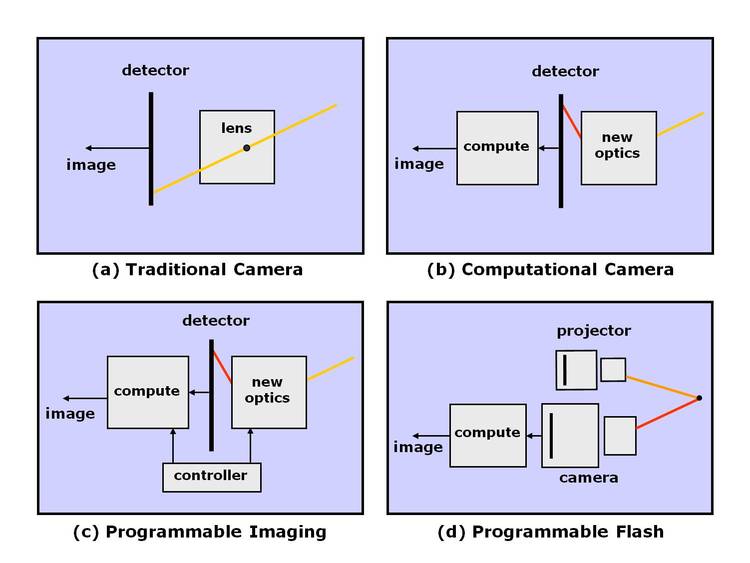
Figure 1:
(a) The traditional camera model, which is based on the camera
obscura. (b) A computational camera uses optical coding followed by
computational decoding to produce new types of images. (c) A
programmable imaging system is a computational camera whose optics
and software can be varied/controlled. (d) The optical coding can
also be done via illumination by means of a programmable flash.
|
||||
| February 2003. Revised: January 2011 | ||||
1. Evolution of the Camera ModelThe Traditional CameraOver the last century, the evolution of the camera has been truly remarkable. However, through this evolution the basic model underlying the camera has remained essentially the same, namely, the camera obscura (Figure 1(a)). The traditional camera has a detector and a standard lens which only captures those principal rays that pass through its center of projection, or effective pinhole, to produce the familiar linear perspective image. In other words, the traditional camera performs a very simple and restrictive sampling of the complete set of rays, or the light field, that resides in any real scene. Computational CamerasA computational camera (Figure 1(b)) uses a combination of novel optics and computations to produce the final image. The novel optics is used to map rays in the light field of the scene to pixels on the detector in some unconventional fashion. For instance, the ray shown in Figure 1(b) has been geometrically redirected by the optics to a different pixel from the one it would have arrived at in the case of a traditional camera. As illustrated by the change in color from yellow to red, the ray could also be photometrically altered by the optics. In all cases, the captured image is optically coded and may not be meaningful in its raw form. The computational module has a model of the optics, which it uses to decode the captured image to produce a new type of image that could benefit a vision system. The vision system could either be a human observing the image or a computer vision system that uses the image to interpret the scene it represents. Programmable Computational CamerasComputational cameras produce images that are fundamentally different from the traditional linear perspective image. However, the hardware and software of each computational camera are typically designed to produce a particular type of image. The nature of this image cannot be altered without significant redesign of the imaging system. A programmable imaging system uses an optical system for forming the image, that can be varied by a controller (Figure 1(c)) in terms of its radiometric and/or geometric properties. When such a change is applied to the optics, the controller also changes the decoding software in the computational module. The result is a single imaging system that can emulate the functionalities of several specialized ones. Such a flexible camera has two major benefits. First, a user is free to change the role of the camera based on his or her needs. Second, it allows us to explore the notion of a purposive camera that, as time progresses, automatically produces the visual information that is most pertinent to the task. In order to give its end-user true flexibility, a programmable imaging system must have an open hardware and software architecture. Programmable IlluminationThe basic function of the camera flash has remained the same since it first became commercially available in the 1930s. It is used to brightly illuminate the camera's field of view during the exposure time of the image detector. It essentially serves as a point light source. Due to the significant technological advances made with respect to digital projectors, the time has arrived for the flash to play a more sophisticated role in the capture of images. The use of a projector-like source as a camera flash is powerful as it provides full brightness and color control over time of each of the 2D set of rays it emits (a projector with a finite aperture actually projects a 4D set of rays but only permits control over two of the dimensions). This enables the camera to project arbitrarily complex illumination patterns onto the scene, capture the corresponding images, and compute information regarding the scene that is not possible to obtain with the traditional flash. In this case, the complete imaging system can still be thought of as a computational camera where captured images are optically coded due to the patterned illumination of the scene (Figure 1(d)). An array of cameras and an array of projectors can be used simultaneously to capture coded measurements of the light field of a scene. Computational decoding of such measurements can facilitate post-capture control of a variety of imaging parameters, including, viewpoint, resolution (spatial, temporal, angular and spectral), depth of field and lighting. |
||||
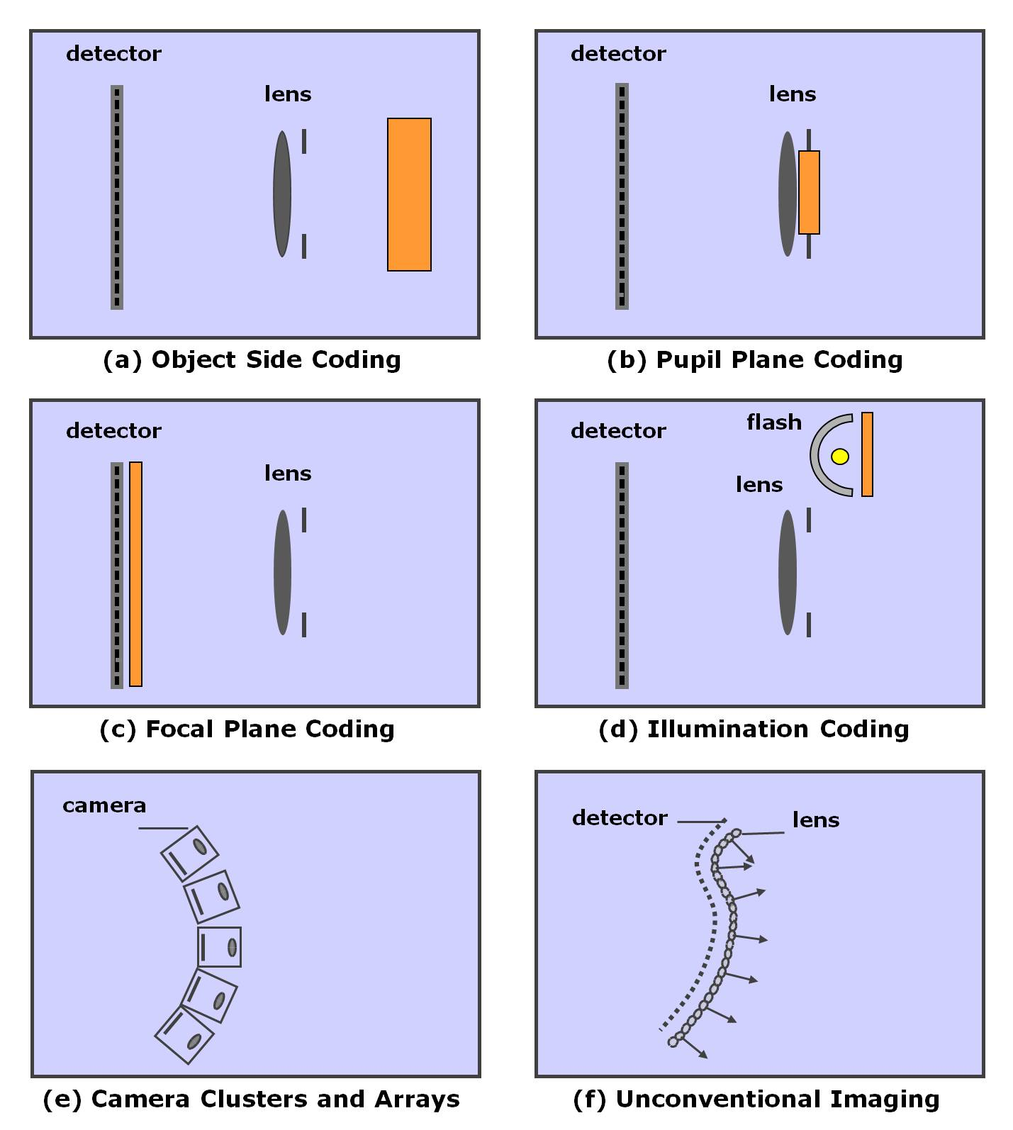
2. Coding ApproachesThe design space for the optics of computational cameras is large. It would be desirable to have a single design methodology that produces an optimized optical system for any given set of imaging specifications. The optimization criterion could incorporate a variety of factors, including performance and complexity. At this point in time, however, such a systematic design approach does not exist. Consequently, as with traditional optics, the design of computational cameras remains part science and part art. The optical coding methods used in today's computational cameras can be broadly classified into the six approaches shown in Figure 2. The first four of these can be viewed as modifications to the traditional camera model. Examples of existing computational cameras that lie in each of the six categories can be found in [Nayar 2011]. Object Side CodingThis is the most convenient way to implement a computational camera, as it only requires optics to be externally attached to a traditional camera (Figure 2(a)). A few examples of this approach include wide angle catadioptric imaging, generalized mosaicing and integral imaging using an externally attached lens or prism array. Object side coding has also been used to develop a variety of "non-central" cameras that do not have a single effective viewpoint but rather a locus of viewpoints. In some cases, the locus of viewpoints is a necessary compromise made to achieve a particular type of image projection and in other cases, such as panoramic stereo, it is a desirable attribute.
Pupil Plane Coding In this case, an optical element is placed at, or close to, the pupil plane of a traditional lens (Figure 2(b)). Examples include the use of phase plates and coded apertures for depth of field extension, the use of coded apertures for enhancing signal-to-noise ratio and resolution, aperture and focus control for depth estimation, aperture splitting for dynamic range extension and image replication, and the use of programmable apertures for viewpoint control and light field capture. Focal Plane CodingHere, an optical element is placed on, or close to, the image detector (Figure 2(c)). In this approach, we also include the use of small physical motions of the image sensor or pixel-wise control of exposure. Examples include the use of lens arrays and attenuation masks for light field imaging, the use of assorted pixel filters for multispectral and high dynamic range imaging, and the use of sensor motion to achieve super-resolution, extended depth of field and motion deblurring. Illumination CodingAs mentioned earlier, by using a spatially and/or temporally controllable flash, captured images can be coded using illumination patterns. This approach enables image coding in ways that are not possible by only altering the imaging optics (Figure 2(d)). Illumination coding has a long history in the field of computer vision - virtually any structured light method or variant of photometric stereo is based on the notion of illumination coding. Recent examples include the use of multiplexed illumination for SNR enhancement and object relighting, and the use of coded illumination patterns for the measurement of light transport in a scene. Camera Clusters and ArraysA number of traditional cameras can be spatially arranged to create new types of images (Figure 2(e)). In this case, these is no explicit optical coding involved. One can view this approach as increasing (in space and/or time) the sampling of the light field. While camera clusters seek to capture wide fields of view with minimal overlap between the fields of view of adjacent cameras, camera arrays capture multiple perspectives of the same scene with large overlap between the fields of view to acquire 3d reconstructions or light fields of the scene. Unconventional Imaging SystemsThese are optical designs that cannot be easily described as modifications to, or collections of, traditional cameras (Figure 2(f)). While we have not seen many well-tested examples of such systems, one can expect novel designs in the decades to come. Examples may include flexible cameras that can be wrapped around objects or incorporated into clothing, networked dust cameras that can be scattered to produce images of volumes of space, and surfaces made of pixels that can both measure and radiate light.
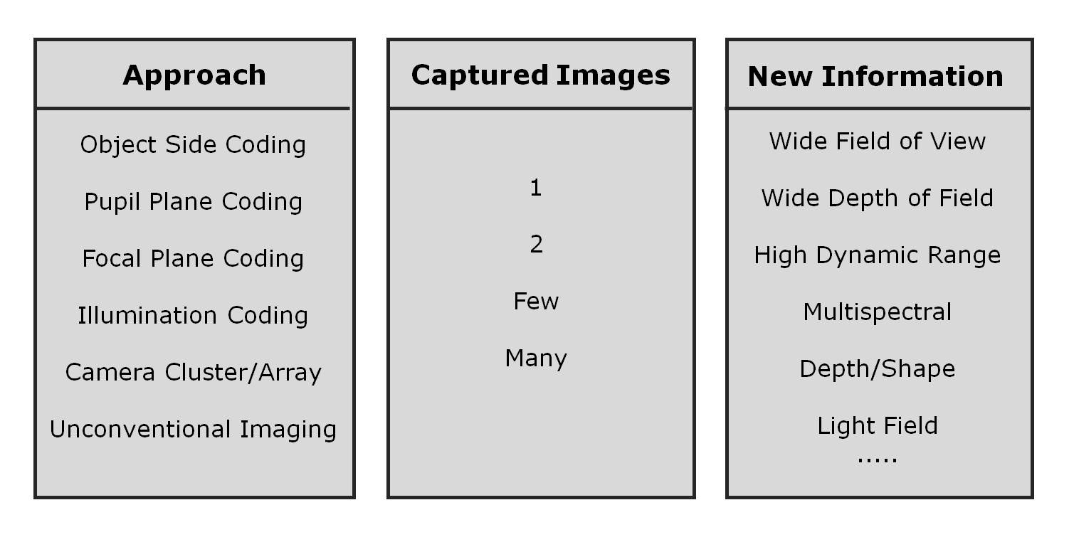
Figure 3 shows a way to characterize computational cameras based on three factors: (a) the technical approach used for coding, (b) the number of images that need to be captured, and (c) the type of information produced. |
||||
3. Benefits of Computational CamerasNew Imaging FunctionalitiesOne motivation for developing computational cameras is to create new imaging functionalities that would be difficult, if not impossible, to achieve using the traditional camera model. The new functionality may come in the form of images with enhanced field of view, spectral resolution, dynamic range, temporal resolution, etc. The new functionality can also manifest in terms of flexibility - the ability to manipulate the optical settings of an image (focus, depth of field, viewpoint, resolution, lighting, etc.) after the image has been captured. Improved Performance-to-Complexity RatioAnother major benefit of computational imaging is that it enables the development of cameras with higher performance-to-complexity ratio than traditional imaging. Camera complexity has yet to be defined in concrete terms. However, one can formulate it as some function of size, weight and cost. In traditional imaging, it is generally accepted that higher performance comes at the cost of complexity. For instance, to increase the resolution of a camera, one needs to increase the number of elements in its lens - this is the only way to combat the aberrations that limit resolution. In contrast, computational imaging allows a designer to shift complexity from hardware to computations. For instance, high image resolution can be achieved by post-processing an image captured with very simple optics (even a single element). |
||||
4. Limits of Computational CamerasThe design of computational cameras may be viewed as choosing an appropriate operating point within a high dimensional parameter space. Some of the parameters are photometric resolution, spatial resolution, temporal resolution, angular resolution, spectral resolution, field of view and F-number. The space could include additional parameters related to the "cost" of the design, such as, size, weight and expense. In general, while making a final design choice to achieve a desired functionality, one is forced to trade-off between the various parameters. In short, as with traditional imaging, there is no "free lunch" with computational cameras. For instance, in the cases of omnidirectional imaging and integral imaging, resolution is traded-off for wider field of view and viewpoint (or focus) control, respectively. Generally, the trade-off made with any given computational camera is straightforward to analyze and quantify. While computational cameras have been shown to enable new imaging functionalities and achieve high performance-to-complexity ratios, it is not known whether computational imaging can be used to break fundamental limits of imaging. For instance, it is not clear that the hard resolution limits imposed by diffraction can be overcome using computations. This is an open question that deserves closer attention. |
||||
5. Related FieldsThe development of computational cameras lies within the larger field of computational imaging. While computational imaging encompasses a wide range of imaging modalities and applications, computational cameras seek to overcome the limits of the traditional camera and impact all fields that use the camera as a source of information. Examples of such fields include photography, computer vision, computer graphics, biometrics, remote sensing and robotics.
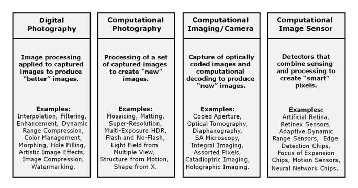
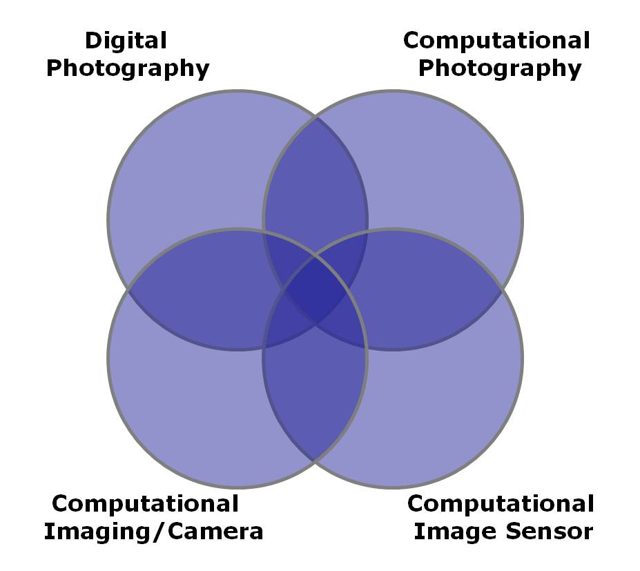
Figure 4 shows one possible way to define the terms digital photography, computational photography, computational imaging/cameras and computational image sensors. The field of computational cameras naturally overlaps the areas of computational photography and computational image sensors (Figure 5). Computational photography includes the development of purely software based methods that seek to process multiple images (which could be taken with even a traditional camera) to produce a new type of image or scene representation. With respect to the computational image sensors, several research teams are developing detectors that can perform image sensing as well as early visual processing.
|
||||
Publications"Computational Cameras: Convergence of Optics and Processing," |
||||
Slides
|
||||
Related Project |